Phillips Curve Definition: The Hidden Link Between Inflation and Unemployment

Economist William Phillips made a groundbreaking find in 1957 that reshaped economic theory. His analysis of UK data spanning almost a century led to the Phillips curve definition, which showed an inverse relationship between inflation and unemployment rates. The relationship appeared true at first and suggested that higher inflation led to lower unemployment. The 1970s challenged this theory when the U.S. economy faced both high inflation and rising unemployment. The economy’s inflation tripled while GDP declined for six consecutive quarters between 1973 and 1975.

This piece explains the Phillips curve concept, its rise, and its role in modern economic policy-making.

What Is the Phillips Curve in Modern Economics?

The Phillips curve is a basic economic model that shows the inverse relationship between inflation and unemployment rates. Economist A.W. Phillips first documented this connection in 1958. The concept has changed substantially through decades of economic research and ground testing.

Definition and Core Concept

The Phillips curve shows a simple trade-off: higher inflation typically means lower unemployment, and the opposite holds true. This relationship suggests that lower unemployment rates come with higher inflation costs. This creates a tough choice for governments and central banks. Economists in the 1960s saw the Phillips curve as a policy menu. It let policymakers pick their preferred mix of unemployment and inflation rates.

Phillips studied 60 years of British data and found a pattern. Wages increased slowly with high unemployment. But when unemployment was low, wages went up faster. Economists Paul Samuelson and Robert Solow later expanded this wage inflation study. They showed the broader connection between price inflation and unemployment.

The Mathematical Relationship Between Inflation and Unemployment

Three main forces guide the modern Phillips curve:

1. Expected inflation – Higher expected inflation typically drives up actual inflation
2. Unemployment gap – The gap between actual unemployment and its natural rate
3. Supply shocks – Outside factors like energy prices that can move the curve

The expectations-increased form of the Phillips curve shows how workers and consumers adjust their future inflation expectations based on current economic conditions. This adjustment creates a difference between short-run and long-run relationships. Understanding this is vital to modern macroeconomics.

The short-run Phillips curve equation looks like this: gP = −f(U − U*) + λ·gP^ex + gUMC

Here, gP means inflation rate, U is unemployment, U* is natural unemployment rate, gP^ex is expected inflation, and gUMC represents supply shocks.

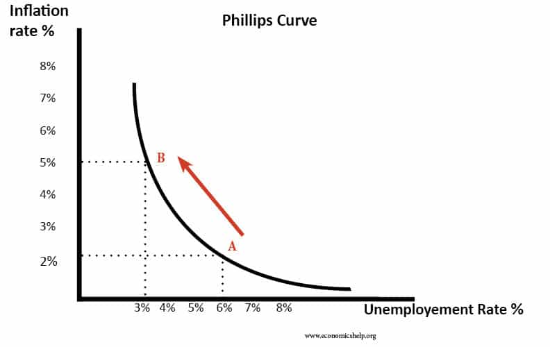
Visual Representation and Interpretation

The Phillips curve appears as a downward-sloping line on a graph. Inflation sits on the Y-axis while unemployment is on the X-axis. This visual helps economists and policymakers understand economic conditions and what their policies might do.

Changes along the curve show shifts in total demand. To cite an instance, point A might show 5% inflation with 4% unemployment. Moving to point B could mean inflation drops to 2% while unemployment rises to 7%.

The whole curve moves when supply shocks hit or inflation expectations change. The 1970s stagflation showed this clearly. The U.S. economy’s GDP fell for six straight quarters while inflation tripled.

Today’s economic theory separates the short-run Phillips curve (SRPC) from the long-run Phillips curve (LRPC). The SRPC keeps the traditional inverse relationship. The LRPC stands vertical at the natural unemployment rate. This suggests no lasting trade-off exists between inflation and unemployment over time.

Short-Run Phillips Curve Mechanics

The short-run Phillips curve mechanics show exactly how the inflation-unemployment relationship works in practice. Unlike long-term economic patterns, the short-run curve reveals what happens when sudden economic changes take place over months or a few years.

Why Unemployment Falls When Inflation Rises

Labor market dynamics are the foundations of this inverse relationship. Businesses see higher revenues when aggregate demand increases in the economy and they just need to produce more goods and services. Companies must hire more workers to increase production, which reduces unemployment.

The labor market tightens as unemployment decreases—leaving fewer workers available to hire. Employers compete for a limited talent pool. Companies offer higher pay to attract qualified candidates because of this competition.

Companies can set higher prices as the economy reaches full capacity. Strong consumer demand lets businesses raise prices without losing customers. The economy experiences inflation when wages and prices both increase.

Price and Wage Setting Behavior

The wage-price spiral drives the Phillips curve mechanism. This process follows several connected steps:

• Workers gain bargaining power and ask for higher wages when unemployment is low
• Companies raise prices to maintain profit margins due to higher labor costs
• Workers ask for more wage increases to keep their purchasing power as prices rise
• This cycle continues until economic conditions change

HR departments set wages based on labor market conditions—they must offer better compensation to motivate workers when unemployment is low. Marketing teams adjust pricing to match these changes and pass costs to consumers. This cycle keeps going until economic conditions shift.

Limitations of the Short-Run Model

The short-run Phillips curve has its most important limitations. The model assumes prices and wages are “sticky” in the short run, meaning they don’t adjust right away to economic changes. This assumption doesn’t work over longer periods.

The model also misses adaptive expectations. Workers and consumers adjust their behavior as they expect inflation—they ask for higher wages early or raise prices before costs increase. The trade-off between inflation and unemployment goes away over time.

The 1970s showed these limitations clearly when stagflation hit—high inflation and high unemployment existed together. This went against the traditional Phillips curve and made economists think about the model differently. Economists now know that while the short-run relationship works temporarily, policymakers can’t use it forever.

Long-Run Phillips Curve Explained

The short-run Phillips curve shows a temporary link between inflation and unemployment, but the long-run analysis paints a completely different picture. We developed this understanding through the work of economists Milton Friedman and Edmund Phelps in the late 1960s. Their research challenges the idea that policymakers can permanently reduce unemployment by accepting higher inflation.

Role of Expectations in Economic Behavior

The biggest difference between short and long-run Phillips curves comes from how people adjust their expectations about future inflation. People and businesses might not see inflation changes coming at first, which lets the short-run trade-off work. All the same, economic players adapt their expectations based on what they experience.

This adaptation process follows a predictable pattern:

1. Workers accept lower real wages when inflation rises unexpectedly because they haven’t adjusted their inflation expectations
2. Workers ask for higher nominal wages to restore their buying power once they notice higher prices
3. Businesses increase prices to maintain profit margins
4. The wage-price spiral continues until expectations fully adjust

Expectations are so vital that economists now call the long-run curve the “Expectations-Augmented Phillips Curve.” Friedman made this clear in his influential 1967 address to the American Economic Association: “There is always a temporary trade-off between inflation and unemployment; there is no permanent trade-off.”

Why No Permanent Trade-Off Exists

The long-run Phillips curve shows up as a vertical line on a graph at what economists call the natural rate of unemployment or NAIRU (Non-Accelerating Inflation Rate of Unemployment). This vertical line shows that unemployment returns to its natural level whatever the inflation rate might be.

The curve becomes vertical because the economy settles at its equilibrium unemployment rate once people fully factor inflation expectations into their decisions. Meltzer puts it simply: “The long-run Phillips curve must be vertical because inflation is a nominal variable and unemployment is a real variable.”

Of course, this has most important implications for policymakers. They can’t keep unemployment below its natural rate through expansionary monetary or fiscal policy. These policies might cut unemployment for a while but lead only to higher inflation without lasting job benefits.

Modern economic forecasting models include this expectations-augmented Phillips curve concept. They recognize that short-term trade-offs exist but fade away as expectations adjust and the economy moves back to its natural unemployment rate.

Real-World Applications for Policymakers

Policymakers worldwide use the Phillips curve to make significant economic decisions. Their approach to this tool has changed noticeably over time. The curve’s real-life applications go beyond theory into actual policy implementation.

Central Bank Decision-Making Framework

Central banks see the Phillips curve as a structural relationship between economic slack and inflation. We used this framework to understand how monetary policies affect financial conditions. These conditions shape economic slack and end up affecting inflation. The European Central Bank (ECB) uses the Phillips curve to analyze economic outlook and create monetary policy. They rely on the transmission mechanism through which standard and non-standard policies affect economic slack.

This relationship helps guide monetary policy decisions. The Federal Open Market Committee (FOMC) meeting transcripts show how the Phillips curve occupies in monetary policy discussions. Former Fed Chair Janet Yellen stated this significance clearly. She noted that “economic theory suggests, and empirical analysis confirms, that such deviations of inflation from trend depend in part on the intensity of resource utilization”.

Fiscal Policy Considerations

Fiscal policy becomes nowhere near as effective when inflation runs high. The economy near full employment means fiscal stimulus either pushes out other spending or results in higher prices. The current mix of high inflation and low unemployment shows the Phillips curve still matters. A small negative effect of fiscal adjustment on demand could help control inflation significantly.

New research shows that:

• Supply disruptions increase inflationary effects of expansionary fiscal policies
• Low economic slack raises inflationary pressure from higher demand
• These factors work together to boost the inflationary effect of fiscal decisions

The Phillips Curve in Economic Forecasting

The Phillips curve’s value in forecasting has faced heavy criticism. Studies compared NAIRU (non-accelerating inflation rate of unemployment) model forecasts to simple naive forecasts. None of the NAIRU forecasts beat simply predicting unchanged inflation. The chances of correctly predicting inflation changes using Phillips curve models matched flipping a coin.

Case Study: Federal Reserve Policy 2015-2020

The Federal Reserve managed to keep its stance that the Phillips curve helped understand inflation during this time. They acknowledged the weaker connection between labor market tightness and inflation. The Fed adjusted its approach instead of dropping the model. Chair Powell noted in 2018 that “almost all participants thought that the Phillips curve remained a useful basis for understanding inflation”.

Wage and price Phillips curve models estimated before 2008 tracked inflation well through 2017. This suggested the low inflation period made sense. The Phillips curve’s slope stayed relatively stable. Only modest flattening occurred since the Great Recession.

Conclusion

The Phillips curve stands as the life-blood of modern economic theory, though experts have substantially changed their interpretation since William Phillips’s original findings. The first model pointed to a simple trade-off between inflation and unemployment. Economic events, especially the 1970s stagflation, showed this relationship was more complex than anyone thought.

Economists now see two different versions of the Phillips curve. The short-run curve reveals temporary trade-offs between inflation and unemployment that wage-price dynamics drive. The long-run curve shows something different – attempts to keep unemployment below its natural rate ended up causing higher inflation.

Central banks across the globe still base their policy decisions on Phillips curve analysis, with much more sophistication than before. The Federal Reserve, European Central Bank, and other institutions use this framework to see how their actions affect inflation and employment. They now look at many more factors like expectations, supply shocks, and structural changes in the economy.

This clearer picture of the Phillips curve explains why we can’t permanently cut unemployment through policies that cause inflation. Good economic management needs us to think over both short-term trade-offs and long-term economic fundamentals.